
Key Concepts & Formulae at a Glance
- The average of a combined collection is (sum of all values) ÷ (total number of values). Simply averaging the averages of the parts works only when every part has the same number of values.
- If Collection 1 has n values with average a, and Collection 2 has m values with average b, the combined average is \(\dfrac{an + bm}{n + m}\).
- When things are mixed, the concentration of the mixture is (total quantity of the substance) ÷ (total quantity of the mixture). Each concentration counts according to how much of that mixture goes in.
- The weighted mean gives each value a weight showing how big or important it is. It is used for averages of averages, mixtures, marks combined in a ratio, and rating systems.
- A stacked bar chart joins the parts of each total end to end, so you can compare the totals and still see the parts that make them up.
- A 100% stacked bar chart draws every total as the same length and splits it in proportion, like a pie chart. It compares shares, not actual amounts.
- A stacked bar chart can always be turned into a 100% stacked bar chart, but not the other way round: the 100% chart doesn't show the totals.
This chapter starts with a simple-looking question: if we know the average height of the seniors and of the juniors in a badminton academy, what is the average height of the whole group? Answering it carefully leads to the weighted mean, an idea Brahmagupta wrote down in his Brāhmasphuṭasiddhānta (c. 628 CE) to find the mean depth of an irregular pit, and which Śrīdharācārya used to work out the purity of gold alloys.
The second half moves from combining numbers to combining them in pictures: cluster-column charts, stacked bar charts and 100% stacked bar charts. It uses family budgets, electricity use, flowers in two gardens and the National Time Use Survey to show which chart answers which kind of question, and which conclusions a chart cannot support.
Weighted Averages: Worked Examples
Answers to the questions asked inside Examples 1–6 (section 10.1), including the first Think and Reflect box.
Think and Reflect
TR(Example 1: 11 trainees — 8 seniors with average height 165.5 cm and 3 juniors with average height 149.33 cm. Method 1 took \(\dfrac{165.5 + 149.33}{2} = 157.415\) cm, while Method 2 added all 11 heights to get 161.09 cm. Shreyas calculated \(\dfrac{(165.5 \times 8) + (149.33 \times 3)}{8 + 3}\).)
Why did Method 1 not work?
Do you understand why this also works? Can you see why 165.5 × 8 gives the sum of the heights of all the seniors and 149.33 × 3 gives the sum of the heights of all the juniors?
Why Method 1 fails. Averaging the two averages treats the seniors' group and the juniors' group as equally important. But there are 8 seniors and only 3 juniors. Each of the 11 trainees should count once, so the seniors' height should have much more say in the overall average. Method 1 gives the 3 juniors as much influence as the 8 seniors, which drags the answer down to 157.415 cm, too low.
Why Shreyas's method works. Average = sum ÷ number of values, so sum = average × number of values.
Sum of the seniors' heights \(= 165.5 \times 8 = 1324\) cm (check: 165 + 169 + 164 + 167 + 170 + 159 + 164 + 166 = 1324).
Sum of the juniors' heights \(= 149.33 \times 3 \approx 448\) cm (check: 146 + 149 + 153 = 448).
So Shreyas's numerator is exactly the total height of all 11 trainees, and his denominator 8 + 3 is exactly the number of trainees:
\(\dfrac{1324 + 448}{11} = \dfrac{1772}{11} = 161.09\) cm, the same as Method 2.
E2Example 2 — Jaspreet recently learnt cycling. She has explored different routes in her town. She tracked how much time she cycled on weekdays over the last 3 weeks. Find the mean time spent cycling per weekday over the last 3 weeks.
Table 10.1: Time spent cycling, in minutes, by JaspreetDay 1 Day 2 Day 3 Day 4 Day 5 Weekly Average Week 1 10 13 10 15 16 12.8 Week 2 14 10 20 17 18 15.8 Week 3 15 18 14 20 23 18
(Method 1 adds the 3 weekly averages and divides by 3, giving 15.53 minutes.)
We saw earlier how Method 1 (badminton example) did not produce the correct value. Why does Method 1 give the correct answer in this case? When does Method 1 work and when does it not work?
| Day 1 | Day 2 | Day 3 | Day 4 | Day 5 | Weekly Average | |
|---|---|---|---|---|---|---|
| Week 1 | 10 | 13 | 10 | 15 | 16 | 12.8 |
| Week 2 | 14 | 10 | 20 | 17 | 18 | 15.8 |
| Week 3 | 15 | 18 | 14 | 20 | 23 | 18 |
| Day 1 | Day 2 | Day 3 | Day 4 | Day 5 | Total | Weekly average | |
|---|---|---|---|---|---|---|---|
| Week 1 | 10 | 13 | 10 | 15 | 16 | 64 | 12.8 |
| Week 2 | 14 | 10 | 20 | 17 | 18 | 79 | 15.8 |
| Week 3 | 15 | 18 | 14 | 20 | 23 | 90 | 18 |
With averages a, b, c and group sizes p, q, r, the combined average is \(\dfrac{ap + bq + cr}{p + q + r}\).
Here every week has the same number of cycling days, p = q = r = 5, so
\(\dfrac{5a + 5b + 5c}{5 + 5 + 5} = \dfrac{5(a + b + c)}{15} = \dfrac{a + b + c}{3}\)
which is exactly Method 1: \(\dfrac{12.8 + 15.8 + 18}{3} = \dfrac{46.6}{3} = 15.53\) minutes. Method 2 gives the same answer: \(\dfrac{64 + 79 + 90}{15} = \dfrac{233}{15} = 15.53\).
In the badminton example the groups had different sizes (8 and 3), so the 5s didn't cancel, and Method 1 failed.
E3Example 3: Two glasses of equal quantities of lemonade are prepared. One glass has 10% jaggery and the other has 20% jaggery. If we mix the lemonade from both glasses, what is the concentration of jaggery in the mixture?
By reasoning. Since both glasses contain equal amounts of lemonade, the mixture will have 15% jaggery — exactly midway between 10% and 20%.
By algebra. Suppose \(y\) is the quantity of lemonade in each glass.
Concentration \(= \dfrac{0.10y + 0.20y}{y + y} = \dfrac{0.30y}{2y} = 0.15 = 15\%\)
E4Example 4 — A bowl of 500 mL lemonade has 10% jaggery. A glass of 200 mL lemonade has 20% jaggery. If we mix the lemonade from the bowl and the glass, what is the concentration of jaggery in the mixture?
Can you estimate what part of the mixture is jaggery? Is it 15%, or is it more or less? Why do you think so?
Estimate. It will be less than 15%. 15% would be right only if equal amounts of the two lemonades were mixed (as in Example 3). Here much more lemonade (500 mL) comes from the 10% bowl, so the mixture will be closer to 10%.
Exact value.
Jaggery in the bowl \(= 500 \times 0.10 = 50\) mL
Jaggery in the glass \(= 200 \times 0.20 = 40\) mL
Concentration \(= \dfrac{50 + 40}{500 + 200} = \dfrac{90}{700} \approx 0.129 \approx 13\%\)
E5Example 5: Brass is an alloy of copper and zinc. Batch A of brass weighs 200 kg of which 70% is copper. Batch B weighs 120 kg of which 50% is copper. Batch C is 45% copper. When all three batches are combined, we get an alloy that is 55% copper. What is the weight of Batch C?
Let \(y\) be the weight (in kg) of Batch C. The concentration of copper in the combined mixture is:
\(0.55 = \dfrac{200 \times 0.7 + 120 \times 0.5 + y \times 0.45}{200 + 120 + y}\)
\(0.55 = \dfrac{140 + 60 + 0.45y}{320 + y} = \dfrac{200 + 0.45y}{320 + y}\)
\(0.55(320 + y) = 200 + 0.45y\)
\(176 + 0.55y = 200 + 0.45y\)
\(0.10y = 24 \implies y = 240\)
Exercise Set 10.1
1The average score of students on a test in Section A is 72 and that of students in Section B is 76. What is the combined average of both the sections given that Section A has 30 students and Section B has 25 students?
Total score of Section A \(= 72 \times 30 = 2160\)
Total score of Section B \(= 76 \times 25 = 1900\)
Combined average \(= \dfrac{2160 + 1900}{30 + 25} = \dfrac{4060}{55} \approx 73.82\)
Check: the answer is closer to 72 than to 76, as expected, because Section A has more students.
2A farmer mixes three equal quantities of fertilisers. The first one contains \(\dfrac{1}{10}\) nitrogen, the second contains \(\dfrac{9}{50}\) nitrogen, and the third contains \(\dfrac{3}{60}\) nitrogen. What is the fraction of nitrogen in the mixture?
The quantities are equal, so the fraction of nitrogen in the mixture is the simple average of the three fractions.
Using the common denominator 300: \(\dfrac{1}{10} = \dfrac{30}{300}\), \(\ \dfrac{9}{50} = \dfrac{54}{300}\), \(\ \dfrac{3}{60} = \dfrac{15}{300}\)
Sum \(= \dfrac{30 + 54 + 15}{300} = \dfrac{99}{300}\)
Fraction of nitrogen \(= \dfrac{99}{300} \div 3 = \dfrac{99}{900} = \dfrac{11}{100}\)
3(Śrīdharācārya, Pāṭīgaṇita, c. 750 CE) In ancient India, Varna was the measure of gold purity. A purity of 16 varṇa meant pure gold; in general, a purity of k varṇa meant that the gold-alloy was \(\dfrac{k}{16}\) gold and the rest impurities. (Now the term used is karat; 16 Varna = 24 karat.)
Suppose a goldsmith melts together three pieces of gold: 9 units at 12 varṇa, 5 units at 10 varṇa, and 17 units at 11 varṇa. Find the purity in varṇa of the combined gold.
The purity of the combined gold is the weighted mean of the purities, weighted by the amount of each piece:
\(\text{Purity} = \dfrac{9 \times 12 + 5 \times 10 + 17 \times 11}{9 + 5 + 17} = \dfrac{108 + 50 + 187}{31} = \dfrac{345}{31} \approx 11.13\) varṇa
(The same answer comes out if we count actual gold: the pieces contain \(\dfrac{108}{16} + \dfrac{50}{16} + \dfrac{187}{16} = \dfrac{345}{16}\) units of pure gold in 31 units of alloy, so the fraction of gold is \(\dfrac{345}{16 \times 31}\), i.e. \(\dfrac{345}{31}\) varṇa.)
4The average rainfall per day in the months of May, June, and July in a certain location are 3.5 mm, 10 mm and 8.7 mm respectively. Write an expression that gives their combined average.
The months have different numbers of days (May 31, June 30, July 31), so each month's average must be weighted by its number of days:
\(\text{Combined average} = \dfrac{3.5 \times 31 + 10 \times 30 + 8.7 \times 31}{31 + 30 + 31}\)
Evaluating: \(\dfrac{108.5 + 300 + 269.7}{92} = \dfrac{678.2}{92} \approx 7.37\) mm per day.
(The simple average \(\dfrac{3.5 + 10 + 8.7}{3} = 7.4\) mm is close but not exact, because the months are nearly, not exactly, the same length.)
5Calculate the concentration of spice mix in these two scenarios.
(i) A 100 mL kashayam/kadha with 5% spice mix, a 200 mL one with 10% spice mix, and a 300 mL one with 15% spice mix are combined.
(ii) A 300 mL kashayam/kadha with 5% spice mix, a 200 mL one with 10% spice mix, and a 100 mL one with 15% spice mix are mixed.
(i) \(\dfrac{100 \times 5 + 200 \times 10 + 300 \times 15}{100 + 200 + 300} = \dfrac{500 + 2000 + 4500}{600} = \dfrac{7000}{600} \approx 11.67\%\)
(ii) \(\dfrac{300 \times 5 + 200 \times 10 + 100 \times 15}{300 + 200 + 100} = \dfrac{1500 + 2000 + 1500}{600} = \dfrac{5000}{600} \approx 8.33\%\)
The same three concentrations give different results because the weights are swapped: in (i) most of the kadha is the strong 15% one, in (ii) most is the mild 5% one.
(ii) \(\dfrac{5000}{600} \approx 8.33\%\)
E6Example 6: Rehmat's marks in Maths are as follows: 60% in internal tests, 64% in the project, 73% in the final exam. The annual percentage score is calculated by combining the internals, project, and final exam in the ratio 3 : 2 : 5. What is Rehmat's annual score in Maths?
If all three had equal weightage (simple average): \(\dfrac{60 + 64 + 73}{3} = \dfrac{197}{3} \approx 65.67\%\).
With the given ratio 3 : 2 : 5, each score is weighted by its importance:
\(\dfrac{60 \times 3 + 64 \times 2 + 73 \times 5}{3 + 2 + 5} = \dfrac{180 + 128 + 365}{10} = \dfrac{673}{10} = 67.3\%\)
Exercise Set 10.2
1Savitri's marks in Kashmiri are as follows: 35 out of 50 in internal tests, 44 out of 60 in the project, and 80 out of 100 in the final exam. The annual percentage score is calculated by combining the internals, project, and final exam in the ratio 3:4:5. Which of the following expression(s) gives her annual score (as a percentage) in Kashmiri?
(i) \(\dfrac{35 \times 3 + 44 \times 4 + 80 \times 5}{3 + 4 + 5}\)
(ii) \(\dfrac{\left(\frac{35}{100}\right) \times 3 + \left(\frac{44}{100}\right) \times 4 + \left(\frac{80}{100}\right) \times 5}{3 + 4 + 5}\)
(iii) \(\dfrac{\left(\frac{35}{50}\right) \times 3 + \left(\frac{44}{60}\right) \times 4 + \left(\frac{80}{100}\right) \times 5}{3 + 4 + 5} \times 100\)
(iv) \(\dfrac{\left(\frac{35}{50} \times 100\right) \times 3 + \left(\frac{44}{60} \times 100\right) \times 4 + \left(\frac{80}{100} \times 100\right) \times 5}{3 + 4 + 5}\)
The three assessments are marked out of different totals (50, 60, 100), so each score must first be turned into a fraction or percentage of its own total. Only then can the weights 3 : 4 : 5 be applied.
(i) Incorrect. It uses the raw marks 35, 44, 80 as if they were all out of the same total.
(ii) Incorrect. It divides 35 and 44 by 100, but they are out of 50 and 60. It also doesn't multiply by 100 at the end, so it isn't a percentage.
(iii) Correct. \(\dfrac{35}{50} = 0.7\), \(\dfrac{44}{60} \approx 0.733\), \(\dfrac{80}{100} = 0.8\) are the right fractions. They are weighted 3 : 4 : 5 and the result is turned into a percentage.
(iv) Correct. It converts each score to a percentage first (70%, 73.33%, 80%) and then takes the weighted mean. This is the same as (iii); the ×100 is just done earlier.
Her score: \(\dfrac{70 \times 3 + 73.33 \times 4 + 80 \times 5}{12} = \dfrac{210 + 293.33 + 400}{12} \approx 75.28\%\)
Exercise Set 10.3
1A stationery shop owner made ₹8000 selling books, of which 30% is the profit amount, and ₹1000 selling book covers, of which 50% is the profit amount. What is the percentage of profit on the total sales?
Profit on books \(= 30\%\) of ₹8000 = ₹2400
Profit on covers \(= 50\%\) of ₹1000 = ₹500
Percentage profit on total sales \(= \dfrac{2400 + 500}{8000 + 1000} \times 100 = \dfrac{2900}{9000} \times 100 \approx 32.22\%\)
This is a weighted mean of 30% and 50% with weights 8000 and 1000, so it lies much closer to 30%. The simple average (40%) would be badly wrong.
2A white stork's migration is tracked. The average daily distance travelled, calculated over 20 days, is 44.5 km. On the 21st day, it flew 55 km. What is the average daily distance travelled over these 21 days? Make a guess before you calculate.
Guess: one day of 55 km is only a little above 44.5 km and is one day among 21, so the average should rise only slightly, to about 45 km.
Total distance in the first 20 days \(= 44.5 \times 20 = 890\) km
Total over 21 days \(= 890 + 55 = 945\) km
New average \(= \dfrac{945}{21} = 45\) km per day
3A 600 mL solution with 5% salt is mixed with a 300 mL solution with 8% sugar. What are the concentrations of salt and sugar in the mixture?
(i) Salt: 5%, Sugar: 8%
(ii) Salt: 13%, Sugar: 3%
(iii) Salt: 6%, Sugar: 6%
(iv) Salt: 5.55%, Sugar: 8.88% (v) Salt: 3.33%, Sugar: 2.67% (vi) Salt: 4.1%, Sugar: 7.08%
Salt in the mixture \(= 5\%\) of 600 mL \(= 30\) mL; sugar \(= 8\%\) of 300 mL \(= 24\) mL. Total volume \(= 600 + 300 = 900\) mL.
Salt concentration \(= \dfrac{30}{900} \times 100 \approx 3.33\%\)
Sugar concentration \(= \dfrac{24}{900} \times 100 \approx 2.67\%\)
Both concentrations go down: each substance is now spread through the whole 900 mL, and each solution adds none of the other substance.
4At a panipuri (golgappa) stall, the concentration of spice in the pani (spiced water) was 8%. Many customers complained that it was too spicy. What quantity of regular water should be mixed into the 10 litres of pani so that the spice level is reduced to \(\left(\dfrac{3}{4}\right)^{\text{th}}\) of the original concentration?
Target concentration \(= \dfrac{3}{4} \times 8\% = 6\%\)
Spice in 10 L of pani \(= 8\%\) of 10 L \(= 0.8\) L. Adding water does not change this amount.
Let w litres of water be added. Then
\(\dfrac{0.8}{10 + w} = 0.06 \;\Rightarrow\; 10 + w = \dfrac{0.8}{0.06} = \dfrac{40}{3} \;\Rightarrow\; w = \dfrac{40}{3} - 10 = \dfrac{10}{3}\)
Check: \(\dfrac{0.8}{10 + \frac{10}{3}} = \dfrac{0.8}{\frac{40}{3}} = 0.06 = 6\%\) ✓
5A physical fitness evaluation is being undertaken. The final marks are calculated by combining the marks for strength, flexibility, and agility in the ratio 4 : 5 : 6. Rashi has scored 60, 65, and 70. Keerthi has scored 55, 65, and 75 respectively.
(i) Find out whose total is more without calculating.
(ii) What are their final marks?
(i) Both have the same flexibility score (65). Rashi is 5 marks ahead in strength (weight 4), and Keerthi is 5 marks ahead in agility (weight 6). The 5 marks Keerthi gains carry more weight than the 5 marks Rashi gains, so Keerthi's final marks are higher.
(ii) Rashi: \(\dfrac{60 \times 4 + 65 \times 5 + 70 \times 6}{4 + 5 + 6} = \dfrac{240 + 325 + 420}{15} = \dfrac{985}{15} \approx 65.67\)
Keerthi: \(\dfrac{55 \times 4 + 65 \times 5 + 75 \times 6}{15} = \dfrac{220 + 325 + 450}{15} = \dfrac{995}{15} \approx 66.33\)
The difference is \(\dfrac{995 - 985}{15} = \dfrac{10}{15}\): exactly \(\dfrac{5 \times (6 - 4)}{15}\), as reasoned in (i).
(ii) Rashi \(= \dfrac{985}{15} \approx 65.67\), Keerthi \(= \dfrac{995}{15} \approx 66.33\).
6A restaurant collected ratings from 10 customers on a scale of 1 to 5. The resulting data is shown in the table below.5 4 3 2 1 Food 5 3 2 0 0 Ambience 0 4 5 1 0 Service 1 2 2 4 1
What is the average rating if the metrics are combined with the weights food : ambience : service = 6 : 5 : 4?
| 5 | 4 | 3 | 2 | 1 | |
|---|---|---|---|---|---|
| Food | 5 | 3 | 2 | 0 | 0 |
| Ambience | 0 | 4 | 5 | 1 | 0 |
| Service | 1 | 2 | 2 | 4 | 1 |
Step 1: average rating for each metric (each is a weighted mean of the star values, weighted by the number of customers):
Food \(= \dfrac{5 \times 5 + 4 \times 3 + 3 \times 2}{10} = \dfrac{43}{10} = 4.3\)
Ambience \(= \dfrac{4 \times 4 + 3 \times 5 + 2 \times 1}{10} = \dfrac{33}{10} = 3.3\)
Service \(= \dfrac{5 \times 1 + 4 \times 2 + 3 \times 2 + 2 \times 4 + 1 \times 1}{10} = \dfrac{28}{10} = 2.8\)
Step 2: combine with weights 6 : 5 : 4
\(\dfrac{4.3 \times 6 + 3.3 \times 5 + 2.8 \times 4}{6 + 5 + 4} = \dfrac{25.8 + 16.5 + 11.2}{15} = \dfrac{53.5}{15} \approx 3.57\)
7The following table shows the weight data of langurs in an animal facility. Without doing any computations, can you tell whether there are more male langurs or more female langurs? Or are they equal in number?
Male langurs Female langurs All langurs Average weight (kg) 16.5 13.8 14.925 Number of langurs 60
(i) Which of the following expression(s) describes the given scenario?
(a) \(\dfrac{16.5x + 13.8y}{x + y} = 14.925\)
(b) \(\dfrac{16.5x + 13.8y}{60} = -14.925\)
(c) \(\dfrac{16.5x + 13.8y}{2} = -14.925\)
(d) \(\dfrac{16.5x + 13.8y}{16.5 + 13.8} = -14.925\)
(ii) Find out how many male langurs are present.
(iii) A female langur weighing 15.2 kg is admitted to the facility. What is the average weight of the female langurs after this?
(iv) Two male langurs weighing 16.9 kg and 16.1 kg are released from the facility. What is the average weight of the male langurs after this?
(v) Now suppose one of the male langurs lost 1 kg of weight. What is the average weight of all the male langurs after this?
| Male langurs | Female langurs | All langurs | |
|---|---|---|---|
| Average weight (kg) | 16.5 | 13.8 | 14.925 |
| Number of langurs | 60 |
Without computing: the overall average 14.925 kg is closer to the females' 13.8 kg than to the males' 16.5 kg (it is 1.125 kg from 13.8 but 1.575 kg from 16.5). So the females pull harder on the average: there are more female langurs.
(i) Let x = number of males, y = number of females.
(a) Correct. Total weight ÷ total number of langurs.
(b) Incorrect. The left side is positive (it is a weighted total divided by 60), but the right side is −14.925, a negative number, so the equation cannot hold. (Without the minus sign it would be the same as (a), since x + y = 60.)
(c) Incorrect. The right side is negative, and dividing by 2 treats it as an average of two things, not of 60 langurs.
(d) Incorrect. The right side is negative, and the denominator must be the number of langurs, not the sum of the two average weights.
(ii) Put y = 60 − x in (a):
\(16.5x + 13.8(60 - x) = 14.925 \times 60\)
\(16.5x + 828 - 13.8x = 895.5\)
\(2.7x = 67.5 \;\Rightarrow\; x = 25\)
So there are 25 male and 35 female langurs.
(iii) Total weight of females \(= 35 \times 13.8 = 483\) kg. After admitting one more: \(\dfrac{483 + 15.2}{36} = \dfrac{498.2}{36} \approx 13.84\) kg.
(iv) Total weight of males \(= 25 \times 16.5 = 412.5\) kg. After releasing two: \(\dfrac{412.5 - 16.9 - 16.1}{23} = \dfrac{379.5}{23} = 16.5\) kg. The average doesn't change, because the two released langurs themselves average \(\dfrac{16.9 + 16.1}{2} = 16.5\) kg.
(v) The total weight of the 23 males drops by 1 kg: \(\dfrac{379.5 - 1}{23} = \dfrac{378.5}{23} \approx 16.46\) kg. The average falls by \(\dfrac{1}{23} \approx 0.04\) kg.
(i) Only (a).
(ii) 25 males.
(iii) ≈ 13.84 kg.
(iv) 16.5 kg (unchanged).
(v) \(\dfrac{378.5}{23} \approx 16.46\) kg.
8Dorjee has collected 1 litre of water from the Dead Sea! Using the information in the table, answer the following questions. A calculator can be used if necessary.
Water Salinity Dead Sea ≈ 34% Other seas and oceans ≈ 3.5% Ground water ≈ 0.01% Purified drinking water ≈ 0.001%
(i) What is the salinity of the mixture if he mixes 1 litre of water from the Dead Sea with 2 litres of purified drinking water?
(ii) Is it possible to mix water from the Dead Sea and purified drinking water to get a mixture with the salinity of groundwater? Why/Why not? What quantity of purified drinking water should Dorjee mix with 1 litre of water from the Dead Sea to get a mixture having the salinity of groundwater?
(iii) Is it possible to mix water from the Dead Sea and groundwater to get a mixture with the salinity of purified drinking water? Why/Why not? What quantity of groundwater should he mix with 1 litre of water from the Dead Sea to get a mixture having the salinity of purified drinking water?
| Water | Salinity |
|---|---|
| Dead Sea | ≈ 34% |
| Other seas and oceans | ≈ 3.5% |
| Ground water | ≈ 0.01% |
| Purified drinking water | ≈ 0.001% |
(i) \(\dfrac{1 \times 34 + 2 \times 0.001}{1 + 2} = \dfrac{34.002}{3} \approx 11.33\%\), still about three times as salty as sea water.
(ii) Yes. A mixture's salinity always lies between the salinities of the parts being mixed. Groundwater's 0.01% lies between 0.001% and 34%, so it can be reached. Let w litres of purified water be mixed with 1 litre of Dead Sea water:
\(\dfrac{34 \times 1 + 0.001w}{1 + w} = 0.01\)
\(34 + 0.001w = 0.01 + 0.01w \;\Rightarrow\; 33.99 = 0.009w \;\Rightarrow\; w \approx 3776.67\)
He would need about 3777 litres (almost 3.8 kilolitres) of purified water for just 1 litre of Dead Sea water.
(iii) No. Purified drinking water (0.001%) is less salty than both Dead Sea water (34%) and groundwater (0.01%). Mixing can never produce a salinity lower than the lowest one being mixed, so no quantity of groundwater will work.
(ii) Yes: about 3777 L of purified water.
(iii) Not possible: 0.001% is below both salinities being mixed.
Stacked Bar Charts: In-Text Questions
Based on Table 10.2: the average weekly expenditure, in rupees (₹), of three families.
| Housing | Food | Education | Transportation | Healthcare | Recreation | Total | |
|---|---|---|---|---|---|---|---|
| Family A | 1940 | 1700 | 1280 | 1200 | 1770 | 535 | 8425 |
| Family B | 1750 | 1546 | 1500 | 1280 | 1210 | 0 | 7286 |
| Family C | 950 | 1700 | 1540 | 1400 | 1300 | 150 | 7040 |
IT(Fig. 10.1: Choice 1 clusters the columns by category; Choice 2 clusters them by family.)
Answer the following questions based on the charts above. Try to answer each question by looking at Choice 1 first, and then Choice 2. Which was easier?
1. Which family spent the least on housing?
2. Which family spent the most on healthcare?
3. Approximately how much did Family A spend on education?
4. Which category did Family B spend most on?
5. Did Family A spend more on food or on healthcare?
Fig. 10.1, Choice 1: clusters by category (redrawn from the textbook)
Fig. 10.1, Choice 2: clusters by family (redrawn from the textbook)
1. Family C (about ₹950, the shortest housing bar).
2. Family A (about ₹1770).
3. About ₹1300 (exactly ₹1280).
4. Housing (about ₹1750).
5. Healthcare (₹1770 against ₹1700 on food).
Which chart was easier? Questions 1–2 compare the families within one category, so Choice 1 (grouped by category) is easier: the three bars you need stand side by side. Questions 4–5 compare categories within one family, so Choice 2 (grouped by family) is easier.
ITFind the answers to the following questions.
6. Which family spent the least amount overall?
7. Approximately how much did Family C spend overall?
8. Approximately what percentage of Family C's expenses were on housing?
Was it as straightforward to answer these questions as the earlier questions? Is there a visualisation that makes it simpler to answer such questions?
Fig. 10.2: A stacked bar chart of the data in Table 10.2 (redrawn from the textbook)
6. Totals: Family A = ₹8425, Family B = ₹7286, Family C = ₹7040. Family C spent the least overall.
7. Family C: 950 + 1700 + 1540 + 1400 + 1300 + 150 = ₹7040 (about ₹7000).
8. \(\dfrac{950}{7040} \times 100 \approx 13.5\%\), roughly one-seventh of the total.
These were not as easy with the cluster charts: you have to read six separate bars and add them up. In the stacked bar chart (Fig. 10.2), the total length of each bar is the family's total, so Question 6 is answered at a glance (Family C's bar is shortest), and Question 8 by comparing the housing piece with the whole bar. The trade-off is that the pieces after the first don't start at 0, so single categories (Questions 1–5) become harder to compare across families.
Exercise Set 10.4
1The following stacked column chart shows the number of animal species in the IUCN Red List, by class, over time.
(Chart — classes: Mammals, Reptiles, Birds, Insects, Amphibians, Molluscs, Fish, Others; years 2007, 2010, 2013, 2016, 2019; column totals 7,851; 9,618; 11,212; 12,630; 14,234.)
(i) What does the number 14,234 on the top of the column 2019 represent?
(ii) Approximately how many reptile species were in the list in 2016?
(iii) Which class(es) of species have seen a relatively small increase in count between 2007 and 2019?
Number of animal species of the IUCN Red List, by class (redrawn from the textbook; segment sizes read from the chart, so approximate)
(i) 14,234 is the total number of animal species of all classes on the IUCN Red List in 2019. It is the height of the whole stacked column, i.e. the sum of all eight coloured pieces.
(ii) In the 2016 column the reptile band (second from the bottom) runs from about 1,150 to about 2,250 on the scale, so there were approximately 1,100 reptile species. (Readings from a chart are approximate, so an answer anywhere from about 1,000 to 1,300 is reasonable.)
(iii) Comparing the thickness of each band in 2007 and 2019: mammals, birds and amphibians have bands of nearly the same thickness in both years, so their counts rose only a little. Fish, insects, molluscs and reptiles grew a lot (the fish band roughly doubled, and the insect band roughly tripled).
(ii) About 1,100 reptile species.
(iii) Mammals, birds and amphibians.
2Test ODI T20 Home 62 100 32 Overseas 172 49 71
The wickets taken by a bowler in International Cricket matches till 2025 are shown in the table. Complete the given stacked bar charts (the bar lengths can be approximate),
(i) comparing the total wickets taken at home vs. overseas:
(ii) the total wickets taken in each format:
| Test | ODI | T20 | |
|---|---|---|---|
| Home | 62 | 100 | 32 |
| Overseas | 172 | 49 | 71 |
(i) Home total = 62 + 100 + 32 = 194; Overseas total = 172 + 49 + 71 = 292. Each bar is split into Test, ODI and T20 pieces.
Wickets taken at home vs. overseas: each bar is split by format.
(ii) Test = 62 + 172 = 234; ODI = 100 + 49 = 149; T20 = 32 + 71 = 103. Each bar is split into Home and Overseas pieces.
Wickets taken in each format: each bar is split into home and overseas.
Chart (i) shows the bowler took many more wickets overseas, mostly in Tests. Chart (ii) shows Tests are his most productive format, while in ODIs most of his wickets came at home.
(ii) Test 234, ODI 149, T20 103.
100% Stacked Bar Charts: Worked Examples
ITTry answering the following question based on the expenditure stacked bar chart you saw earlier:
Which family has the smallest share of their total expenditure towards healthcare?
Was it easy?
If not, what visualisation can help answer such questions easily?
Fig. 10.3: Pie charts of data of each family in Table 10.2 (redrawn from the textbook)
Fig. 10.4: A 100% stacked bar chart of data in Table 10.2 (redrawn from the textbook)
Healthcare shares: Family A \(= \dfrac{1770}{8425} \approx 21.0\%\), Family B \(= \dfrac{1210}{7286} \approx 16.6\%\), Family C \(= \dfrac{1300}{7040} \approx 18.5\%\).
The ordinary stacked bar chart makes this hard: the three bars have different lengths and the healthcare pieces start at different points, so you can't compare shares by eye. Pie charts (Fig. 10.3) or a 100% stacked bar chart (Fig. 10.4) show proportions directly. In the 100% chart every bar is the same length, so the piece lengths are the shares.
E7Example 7 — The average category-wise daily electricity consumption of a house, in kWh, in 2005 and 2025 is shown in the table below. The corresponding stacked bar chart is also shown.
Lighting Cooling Kitchen appliances Other appliances 2005 360 300 120 220 2025 220 800 460 520
Make the corresponding 100% stacked bar chart.
What do you observe? What do you find interesting in the data/graphs? Discuss with others.
| Lighting | Cooling | Kitchen appliances | Other appliances | |
|---|---|---|---|---|
| 2005 | 360 | 300 | 120 | 220 |
| 2025 | 220 | 800 | 460 | 520 |
Stacked bar chart shown with Example 7 (redrawn from the textbook)
2005: total = 360 + 300 + 120 + 220 = 1000. Shares: Lighting \(\dfrac{360}{1000} = 36\%\), Cooling 30%, Kitchen 12%, Other 22%.
2025: total = 220 + 800 + 460 + 520 = 2000. Shares: Lighting \(\dfrac{220}{2000} = 11\%\), Cooling \(\dfrac{800}{2000} = 40\%\), Kitchen \(\dfrac{460}{2000} = 23\%\), Other \(\dfrac{520}{2000} = 26\%\).
100% stacked bar chart of daily electricity use, 2005 and 2025.
Observations:
• Total use has doubled (1000 → 2000). The ordinary stacked chart shows this; the 100% chart hides it.
• Lighting fell in actual use (360 → 220) and in share (36% → 11%). More efficient lighting, such as LED bulbs, could explain this.
• Cooling is now the biggest share (30% → 40%). Its actual use grew more than 2.5 times (300 → 800).
• Kitchen appliances almost quadrupled (120 → 460), and their share nearly doubled (12% → 23%).
E8Example 8 — The 100% stacked bar below compares the proportion of flowers blooming in Fatima's garden and Naveen's garden across seasons.
(Chart — Fatima: Summer 50%, Monsoon 30%, Winter 20%; Naveen: Summer 40%, Monsoon 25%, Winter 35%.)
Which of the following statements can be inferred from this chart?
(i) In Fatima's garden, there were more blooms in the summer than in the monsoon.
(ii) In summer, Fatima's garden had more blooms than Naveen's garden.
(iii) In winter, Fatima's garden had fewer blooms than Naveen's garden.
(iv) The total number of flowers, across seasons, is the same in both gardens but it varies in each season.
(Hint: Find out the blooms per season in each garden if both the gardens had the same total number of blooms over the year. Similarly find out what happens if the totals are very different.)
Proportion of flowers that bloomed across seasons (redrawn from the textbook)
(i) Can be inferred. It compares two parts of the same bar (the same total): 50% of Fatima's flowers is more than 30% of Fatima's flowers.
(ii) Cannot be inferred. It compares across gardens, but the chart doesn't show the totals. Case 1: Fatima 210 flowers, Naveen 120, so summer blooms are 105 vs 48 and Fatima has more. Case 2: Fatima 180, Naveen 240, so summer blooms are 90 vs 96 and Naveen has more. Both cases give the same 100% chart.
Rows marked 1 = Case 1, 2 = Case 2: the same 100% chart can come from very different numbers of flowers
(iii) Cannot be inferred, for the same reason. In Case 1 both gardens had 42 winter blooms, even though the percentages (20% and 35%) are different.
(iv) Cannot be inferred. Every bar in a 100% chart has the same length whatever its total, so the chart says nothing about whether the totals are equal.
Think and Reflect
TR1. What does this say about the scope of the stacked bars and 100% stacked bars?
2. Given a stacked bar chart can we make a corresponding 100% stacked bar chart?
3. Given a 100% stacked bar chart can we make a corresponding stacked bar chart?
4. What kind of inferences or comparisons can be made from a stacked bar chart and in a 100% stacked bar chart?
1. A stacked bar shows actual amounts, so it supports questions about totals and about how much. A 100% stacked bar shows only proportions, so it supports questions about what share or what fraction, but never about how many.
2. Yes. From a stacked bar we can read each part and the total, and divide: share = part ÷ total × 100 (as in Example 7).
3. No, not by itself. The 100% chart has lost the totals (Cases 1 and 2 in Example 8 give the same 100% chart). If the totals are also given, we can rebuild it: part = share × total.
4. Stacked bar: compare totals across bars, estimate actual sizes of parts, and see a part's rough share of its own bar. 100% stacked bar: compare the shares of categories within a bar and across bars. It cannot compare actual amounts or totals across bars.
E9Example 9 — The following chart shows the time spent on different activities in a day by the average Indian. What do you notice? What do you wonder about?
(Fig. 10.5, National Time Use Survey 2024 — Sleep 34%, Personal care 13%, Paid work 10%, Unpaid work & care 11%, Learning 5%, Leisure, social & travel 27%.)
Fig. 10.5: Time spent on different activities in a day by an average Indian (values are rounded off). Source: National Time Use Survey 2024. Redrawn from the textbook.
Converting to hours (out of 24):
| Activity | Share | ≈ Hours per day |
|---|---|---|
| Sleep | 34% | 8.2 |
| Leisure, social & travel | 27% | 6.5 |
| Personal care | 13% | 3.1 |
| Unpaid work & care | 11% | 2.6 |
| Paid work | 10% | 2.4 |
| Learning | 5% | 1.2 |
Noticing: about a third of the day goes to sleep, and leisure/social/travel is the next biggest piece. Paid work is only about 2.4 hours. That seems low, but it is an average over everyone, including children, students, the elderly and people who don't do paid work. Similarly, learning is only about 1.2 hours because most adults aren't studying.
Wondering: How different is this for children, working adults or the elderly? For women and men? For rural and urban people? These questions lead naturally to the age-wise breakdown in Fig. 10.6. An average of a very diverse group can hide big differences inside it.
Think and Reflect
TRFig. 10.6 (Time use by age group): Children (6–14): Sleep 38%, Personal care 13%, Learning 22%, Leisure 26% (plus a very thin unlabelled sliver of unpaid work, about 1%). Youth (15–24): Sleep 34%, Personal care 13%, Paid work 7%, Unpaid work 9%, Learning 11%, Leisure 26%. Adults (25–59): Sleep 32%, Personal care 13%, Paid work 14%, Unpaid work 15%, Leisure 26%. Elderly (60+): Sleep 37%, Personal care 14%, Paid work 7%, Unpaid work 9%, Leisure 33%.
1. What do you find interesting in the chart above? What can you infer? Discuss.
2. Do you remember the sleep time over age trend that you studied last year? Does that trend align with this chart?
3. Can you explain why the learning time of people in the age group 15 - 24 has reduced significantly compared to that of the age group 6 - 14?
4. Do adults spend about an equal amount of time in paid and unpaid work? What do you think?
Fig. 10.6: Age-wise grouping of data (values are rounded off). Source: National Time Use Survey 2024. Redrawn from the textbook.
1. Some things to notice:
• Personal care stays at about 13–14% (≈ 3 h) in every group.
• Leisure is about 26% for everyone under 60, then rises to 33% (≈ 8 h) for the elderly.
• Learning takes 22% (≈ 5.3 h) of a child's day, but work (paid + unpaid) takes 29% (≈ 7 h) of an adult's day.
Inference: what fills the day changes a lot with age, which the single "average Indian" bar in Fig. 10.5 completely hid.
2. Sleep: children 38% (≈ 9.1 h), youth 34% (≈ 8.2 h), adults 32% (≈ 7.7 h), elderly 37% (≈ 8.9 h). From childhood to adulthood sleep time decreases with age, which fits the usual trend. For the elderly it goes up again, perhaps because rest and time in bed increase after people stop working.
3. Many people in the 15–24 group finish school or college and start working or take on household responsibilities. Learning falls from 22% to 11% (≈ 5.3 h to ≈ 2.6 h), while paid work (7%) and unpaid work (9%) appear for the first time.
4. On average, yes: paid work 14% (≈ 3.4 h) and unpaid work & care 15% (≈ 3.6 h) are nearly equal. But this is an average over all adults. It may hide the fact that some people (for example, many women) do mostly unpaid work while others do mostly paid work. Breaking the data down by gender would tell us.
TRDo you remember the "What Can A Strip Say?" activity from last year? In each strip, if we club the tiny strips belonging to each activity together, will we get a 100% stacked bar chart like the one in Fig. 10.6?
Yes. Each day-strip represents 24 hours, split into many small pieces as activities change through the day. If we collect all the pieces for the same activity (all the sleep pieces, all the learning pieces, and so on) and put them together, we get one bar split into activities. That is a stacked bar whose total is always 24 hours.
Since every person's total is the same 24 hours, these bars all have the same length. So it is a stacked bar chart and a 100% stacked bar chart at once, just like Fig. 10.6. The one difference is that Fig. 10.6 shows the average for each age group, so we would need to average the clubbed strips of everyone in that group.
Exercise Set 10.5
1The smart watch data of 5 people was tracked from Monday to Friday. The recorded data tells us how many hours each person spent lying down, sitting, and standing or moving around, etc., as shown in the following table.
Table 10.3: Average number of hours spent per day (Monday–Friday) lying down, sitting, and standing or moving around, etc., of 5 peopleLying down Sitting Standing or Moving around etc. Pavani (Patient) 20 3 1 Raghu (Nurse) 7 4 13 Zakir (Teacher) 8 6 10 Sahana (Student) Julie (__________) 8 10 6
(i) How much time does Sahana spend per day in each of these body-states? Make a reasonable guess and fill her row in the table.
(ii) Guess what activity or work Julie could be engaged in based on the data. Find out what your classmates' guesses are.
(iii) Complete the chart below based on the tabular data.
| Lying down | Sitting | Standing or Moving around etc. | |
|---|---|---|---|
| Pavani (Patient) | 20 | 3 | 1 |
| Raghu (Nurse) | 7 | 4 | 13 |
| Zakir (Teacher) | 8 | 6 | 10 |
| Sahana (Student) | |||
| Julie (__________) | 8 | 10 | 6 |
(i) A school student sleeps about 8 hours and sits for most of the school day, homework and meals. A reasonable guess (the three must add to 24):
Sahana: Lying down 8 h, Sitting 9 h, Standing/moving 7 h (total 24 h). Other sensible guesses are fine too, e.g. 9, 9, 6.
(ii) Julie sits for 10 hours a day, much more than anyone else, and stands or moves for only 6. She could be an office worker (for example, a computer programmer or accountant), a bank cashier, a receptionist or a bus/taxi driver. Answers may vary; what matters is that the job involves long hours of sitting.
(iii) Each person's total is 24 h, so each share = hours ÷ 24 × 100:
| Person | Lying down | Sitting | Standing/moving |
|---|---|---|---|
| Pavani | 20 h (83.3%) | 3 h (12.5%) | 1 h (4.2%) |
| Raghu | 7 h (29.2%) | 4 h (16.7%) | 13 h (54.2%) |
| Zakir | 8 h (33.3%) | 6 h (25%) | 10 h (41.7%) |
| Sahana | 8 h (33.3%) | 9 h (37.5%) | 7 h (29.2%) |
| Julie | 8 h (33.3%) | 10 h (41.7%) | 6 h (25%) |
Completed 100% stacked bar chart (Sahana's row uses the guessed values 8, 9, 7 hours).
(ii) A desk job such as an office worker (answers vary).
(iii) Sahana's bar: 33.3% | 37.5% | 29.2%, drawn as above.
Think and Reflect
TR1. Will the bars look similar if a different teacher's data is considered instead of Zakir's?
2. Will the bars look different if the data for all 7 days of the week is considered?
3. Some bars in the chart may also match people doing other kinds of work/activities. Can you think of any? Discuss.
1. Broadly similar, but not identical. Most teachers stand while teaching and sleep about 7–8 hours, so the overall pattern (large standing share, moderate sitting) would be similar. The exact lengths would change: a teacher who spends more time correcting notebooks or teaching online would have a longer "sitting" piece. One person's data is only one example.
2. Probably yes. On Saturday and Sunday most people don't go to school or work, so a teacher or a student would likely sit or rest more and stand less. Including the weekend would change the averages, making the lying-down and sitting pieces larger for Zakir and Sahana. Pavani the patient's bar would change the least.
3. Some examples:
• A bar like Pavani's (mostly lying down) could match someone recovering from an illness or injury.
• A bar like Raghu's (mostly standing/moving) could match a shopkeeper, waiter, traffic police officer, farmer, construction worker or sports coach.
• A bar like Julie's (mostly sitting) could match a software engineer, accountant, tailor or bus driver.
End-of-Chapter Exercises
1In cricket, the run rate is the average number of runs scored per over. In a T20 match, a team scored 6 runs in the first over making the run rate 6.
(i) In the second over they scored 12 runs. What is the run rate now?
(ii) After Over 19, their run rate was 6. What is the run rate after 20 overs given the team made 12 runs in the last over?
(i) Runs = 6 + 12 = 18 in 2 overs. Run rate \(= \dfrac{18}{2} = 9\).
(ii) Runs after 19 overs \(= 6 \times 19 = 114\). After 20 overs: \(114 + 12 = 126\). Run rate \(= \dfrac{126}{20} = 6.3\).
Notice how much one over moves the run rate in (i) (from 6 to 9) compared with (ii) (from 6 to 6.3). An extra value affects an average less when there are already many values.
(ii) Run rate = \(\dfrac{126}{20} = 6.3\).
2Five friends who play badminton surveyed the city and collected the price of shuttlecocks across brands and types (Nylon and Feather). The following is the list of the prices, in rupees (₹), that each one compiled.
Yusuf: 40(N), 105(N), 383(F), 108(N), 165(F), 116(F)
Srikanth: 194(N), 85(N), 93(N), 121(N)
Kashvi: 49(N), 297(F), 105(N), 275(F), 40(N)
Prasanna: 124(N), 333(F), 182(N), 258(F)
Gracy: 220(F), 458(F), 129(F), 183(N)
Can you describe a way they can work together to find the average price of a shuttlecock across types?
(i) Each one calculated the average of the prices they had gathered. Suppose these are \(a_y, a_s, a_k, a_p, a_g\) respectively. Write an expression that gives the combined average.
(ii) Suppose \(a_n, a_f\) are the average prices of the nylon shuttlecocks and the feather shuttlecocks, respectively. Write an expression that gives the average price of a shuttlecock. Will this be equal to the answer we got using the method in the previous part?
(i) The friends collected different numbers of prices: Yusuf 6, Srikanth 4, Kashvi 5, Prasanna 4, Gracy 4 (total 23). Each average is weighted by its count:
\(\text{Combined average} = \dfrac{6a_y + 4a_s + 5a_k + 4a_p + 4a_g}{6 + 4 + 5 + 4 + 4} = \dfrac{6a_y + 4a_s + 5a_k + 4a_p + 4a_g}{23}\)
(ii) Counting by type: 13 nylon and 10 feather shuttlecocks (13 + 10 = 23).
\(\text{Average price} = \dfrac{13a_n + 10a_f}{13 + 10} = \dfrac{13a_n + 10a_f}{23}\)
Yes, it is equal. Both expressions work out to (sum of all 23 prices) ÷ 23. They just group the same 23 prices differently, by friend or by type.
Checking with the data: nylon total = ₹1429, so \(a_n = \dfrac{1429}{13} \approx 109.92\). Feather total = ₹2634, so \(a_f = \dfrac{2634}{10} = 263.4\). Average \(= \dfrac{1429 + 2634}{23} = \dfrac{4063}{23} \approx 176.65\) rupees either way. (The unweighted \(\dfrac{a_n + a_f}{2} \approx 186.66\) rupees would be wrong, because there are more nylon shuttlecocks.)
(ii) \(\dfrac{13a_n + 10a_f}{23}\): equal to (i), both ≈ ₹176.65.
3Shreyas holds 25 shares of a company at an average price of ₹150 and Vaishnavi holds 5 shares of the same company at an average price of ₹150.
(i) Shreyas buys 10 shares of this company at a price of ₹30 each. What is the average price per share for him after the purchase?
(ii) Vaishnavi buys some shares of this company at a price of ₹30 each and the average price per share for her after the purchase is ₹70. How many shares did she buy?
(i) \(\dfrac{25 \times 150 + 10 \times 30}{25 + 10} = \dfrac{3750 + 300}{35} = \dfrac{4050}{35} \approx 115.71\)
(ii) Let her buy k shares:
\(\dfrac{5 \times 150 + 30k}{5 + k} = 70\)
\(750 + 30k = 350 + 70k \;\Rightarrow\; 400 = 40k \;\Rightarrow\; k = 10\)
Check: \(\dfrac{750 + 300}{15} = \dfrac{1050}{15} = 70\) ✓. Buying 10 cheap shares lowers Vaishnavi's average far more than Shreyas's, because she started with only 5 shares.
(ii) She bought 10 shares.
4(Pṛthūdakasvāmī, commentary on Brahmagupta's Brāhmasphuṭasiddhānta, c. 864 CE) A "hasta" (meaning "forearm") refers to a unit of length measuring around 18 inches. A pool 30 hastas long is dug to different depths along its length. It is divided into 5 sections having lengths 4, 5, 6, 7, and 8 hastas, and is dug to depths of 9, 7, 7, 3, and 2 hastas, respectively. Find the mean depth of the pool.
Each depth is weighted by the length of its section (Brahmagupta's formula):
\(\text{Mean depth} = \dfrac{4 \times 9 + 5 \times 7 + 6 \times 7 + 7 \times 3 + 8 \times 2}{4 + 5 + 6 + 7 + 8}\)
\(= \dfrac{36 + 35 + 42 + 21 + 16}{30} = \dfrac{150}{30} = 5\) hastas
(The simple average of the depths, \(\dfrac{28}{5} = 5.6\), would be too high, because the deepest parts are the shortest sections.)
5Suvarna had purchased 1g gold at ₹15k (short for ₹15,000). This is shown by point O denoting the average price of gold that she possesses. Six different scenarios are given below for her next transaction. For each scenario estimate and mark the average price of gold she will have after the transaction.
(i) Purchase 1g gold at ₹30k
(ii) Purchase 2g gold at ₹30k
(iii) Purchase 1g gold at ₹10k
(iv) Purchase 10g gold at ₹10k
(v) Purchase 0.5g gold at ₹30k
(vi) Purchase 0.5g gold at ₹15k
New average (in ₹k per g) \(= \dfrac{1 \times 15 + w \times p}{1 + w}\), where w grams are bought at price p.
(i) \(\dfrac{15 + 30}{2} = 22.5\) (exactly midway: equal amounts)
(ii) \(\dfrac{15 + 60}{3} = 25\) (closer to 30: twice as much bought at 30)
(iii) \(\dfrac{15 + 10}{2} = 12.5\) (midway)
(iv) \(\dfrac{15 + 100}{11} = \dfrac{115}{11} \approx 10.45\) (very close to 10: 10 g against 1 g)
(v) \(\dfrac{15 + 15}{1.5} = 20\) (closer to 15: only half a gram at 30)
(vi) \(\dfrac{15 + 7.5}{1.5} = 15\) (no change: bought at the same price)
New average price (₹k per gram) after each transaction; O is the starting average, 15.
(ii) ₹25k
(iii) ₹12.5k
(iv) ≈ ₹10.45k
(v) ₹20k
(vi) ₹15k (unchanged)
6Given some data with corresponding weights, how would the weighted average change if all the weights are doubled? If required, experiment with some data. What do you observe? Justify your answer using algebra.
Experiment. Values 60, 64, 73 with weights 3, 2, 5: \(\dfrac{180 + 128 + 365}{10} = 67.3\). With doubled weights 6, 4, 10: \(\dfrac{360 + 256 + 730}{20} = \dfrac{1346}{20} = 67.3\). No change.
Algebra. With weights \(2w_1, 2w_2, \ldots, 2w_n\):
\(\dfrac{2w_1x_1 + 2w_2x_2 + \cdots + 2w_nx_n}{2w_1 + 2w_2 + \cdots + 2w_n} = \dfrac{2(w_1x_1 + w_2x_2 + \cdots + w_nx_n)}{2(w_1 + w_2 + \cdots + w_n)} = \dfrac{w_1x_1 + \cdots + w_nx_n}{w_1 + \cdots + w_n}\)
The factor 2 cancels. The same happens when all weights are multiplied by any positive number k. Only the ratio of the weights matters, which is why weights like 3 : 2 : 5 can be written as a ratio.
7Answer the following questions based on the graph.
(Graph — cumulative number of objects currently orbiting Earth, by year of launch (as of Apr. 24, 2026), split into payload objects and other objects.)
(i) In 2003, approximately how many total objects were found orbiting Earth in space? In what year did this number double?
(ii) Find the approximate number and share of payload objects and other objects in the year 2025.
(iii) What can you say about the number of payload objects over time, and the number of other objects over time? What can you say about the share of payload objects over time, and the share of other objects over time?
Cumulative number of objects currently orbiting Earth, by year of launch/separation (as of Apr. 24, 2026). * Former transport good of a rocket (e.g., spaceship, satellite). ** Space mission components, debris, rocket stages. Source: J. McDowell, General Catalogue of Artificial Space Objects, Release 1.8.0 (2026). Redrawn from the textbook; bar heights read from the chart, so approximate.
(i) The 2003 column reaches about 10,000 objects. Double that is about 20,000, which the columns reach around 2021.
(ii) In 2025 the column reaches about 33,000 in total, with the payload (light green) part up to about 17,000.
| 2025 | Approx. number | Approx. share |
|---|---|---|
| Payload objects | ≈ 17,000 | ≈ 51% |
| Other objects | ≈ 16,000 | ≈ 49% |
| Total | ≈ 33,000 | 100% |
(Readings from a graph are approximate; answers close to these are fine.)
(iii) Numbers: other objects (debris, rocket stages and so on) have grown steadily since the 1960s, with a sudden jump around 2007. Payload objects grew slowly for about 50 years, then shot up after about 2019.
Shares: for most of the period payload objects were only a small share, roughly one-fifth to one-quarter of all objects (e.g. ≈ 2,300 of ≈ 10,000 in 2003). After about 2019 the payload share rose rapidly to about half by 2025, and the share of other objects fell correspondingly. Even so, the number of other objects kept increasing.
(ii) 2025: payload ≈ 17,000 (≈ 51%), other ≈ 16,000 (≈ 49%).
(iii) Both numbers rise, payload very sharply after ≈ 2019; the payload share jumped from about ¼ to about ½.
8Observe the following infographic.
("What Percentage of Schools have a Playground?" — e.g. Haryana 90%, Uttarakhand 78%, Arunachal Pradesh 68%, Punjab 98%, Dadra & Nagar Haveli and Daman & Diu 99.8%, Maharashtra 93%, Telangana 74%.)
(i) Identify the correct inference(s) from the statements given.
(a) More schools have a playground in Haryana compared to Uttarakhand.
(b) Approximately every 2 out of 3 schools in Arunachal Pradesh have a playground.
(c) Punjab has the highest number of schools with a playground.
(d) Suppose it is given that Maharashtra has more schools than Telangana. Then the number of schools having a playground is more in Maharashtra.
(ii) Using the information given, can we find the nation-wide percentage of schools with a playground? If not, what additional information is needed?
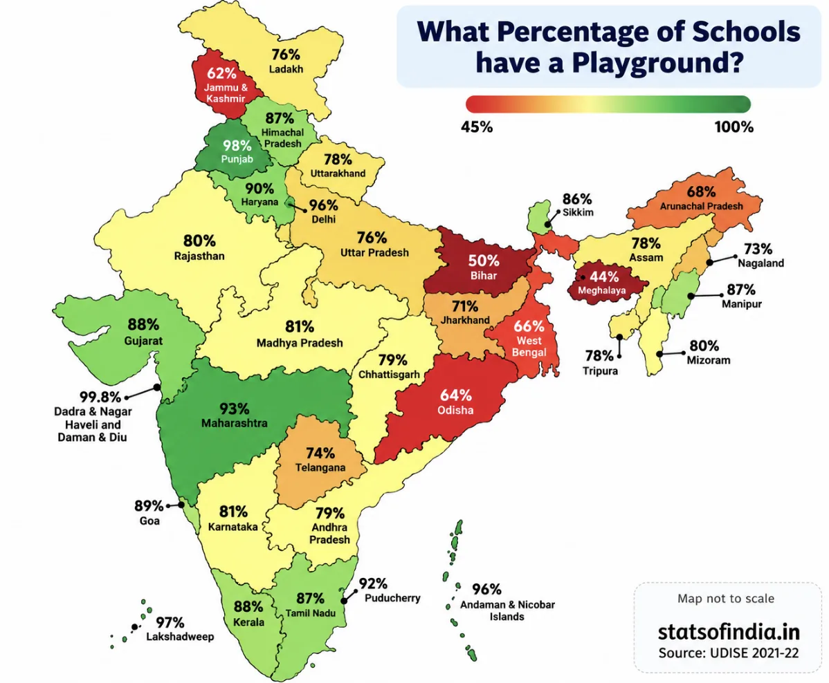
What percentage of schools have a playground? Source: UDISE 2021-22 (statsofindia.in). Map not to scale.
(i)
(a) Cannot be inferred. Haryana's percentage (90%) is higher than Uttarakhand's (78%), but the statement is about the number of schools. Without the total number of schools in each state, we can't compare numbers.
(b) Correct. Arunachal Pradesh shows 68%, and 2 out of 3 is \(\dfrac{2}{3} \approx 67\%\).
(c) Incorrect. The map gives percentages, not numbers, so "highest number" can't be read from it. Even by percentage, Punjab (98%) is not the highest: Dadra & Nagar Haveli and Daman & Diu shows 99.8%.
(d) Correct. Maharashtra has a higher percentage (93% vs 74%) and, as given, more schools. A bigger share of a bigger number is a bigger number.
(ii) No. The nation-wide percentage is a weighted average of the state percentages, weighted by the number of schools in each state. A simple average of the percentages would treat a small union territory the same as a large state. The additional information needed is the number of schools in each state/UT. Then
\(\text{National \%} = \dfrac{\sum (\text{no. of schools in state}) \times (\text{state \%})}{\sum (\text{no. of schools in state})}\)
(ii) No: we need the number of schools in each state, to take a weighted average of the percentages.
9Decision Dilemma:
(i) Which of the plays would you choose to watch based on the following chart?
(Chart: "Share of ratings of three plays", a 100% stacked bar.)
(ii) The corresponding stacked bar chart is shown below. Would you change your decision after looking at this chart? Why/Why not? Discuss.
(Chart: "Ratings of three plays", a stacked bar.)
Share of ratings of three plays (redrawn from the textbook; shares read from the chart)
Ratings of three plays (redrawn from the textbook; counts read from the chart, so approximate)
Approximate readings from the two charts:
| Play | 5★ | 4★ | 3★ | 2★ | 1★ | ≈ No. of ratings |
|---|---|---|---|---|---|---|
| A | 29% | 43% | 14% | 2% | 12% | ≈ 210 |
| B | 24% | 48% | 15% | 3% | 10% | ≈ 920 |
| C | 40% | 13% | 4% | 11% | 32% | ≈ 380 |
(i) From the 100% chart alone, Play A looks like the best choice. About 72% of its ratings are 4★ or 5★ (the same as B), and it has a slightly larger 5★ share than B. Estimated average ratings: A ≈ 3.75, B ≈ 3.73, C ≈ 3.18. Play C has the most 5★ ratings but also about one-third 1★ ratings: people either love it or dislike it.
(ii) The stacked chart shows the actual number of ratings. Play B has about 920 ratings, more than four times Play A's (about 210). Its shares are nearly the same as A's but come from far more people, so B's rating is more reliable. A handful of extra ratings could change A's shares noticeably. Many people would therefore switch to Play B. (Someone who likes bold, unusual shows might still choose C for its large 5★ share, knowing the risk.)
(ii) Yes, many would switch to Play B: equally good shares, but based on about 920 ratings versus about 210, so it is more trustworthy.
10A triathlon is an endurance race consisting of swimming 3.8 km, cycling 180 km, and running 42.2 km. Athletes compete for the fastest overall time, completing each segment in that order. The following table shows the finish time of 3 athletes in each segment.
Table 10.4: Finish time of three athletes in each segment of a triathlon race (values in hh:mm)Swimming Cycling Running Athlete 1 01:08 05:00 03:15 Athlete 2 01:05 05:10 03:35 Athlete 3 01:22 05:55 03:50
(i) What is a suitable representation of this data—a stacked bar chart or a 100% stacked bar chart? Why do you think so?
(ii) Suppose a 100% stacked bar chart is drawn. Which of the following question(s) can be answered by looking at just that chart?
(a) Who finished the race first?
(b) Approximately what fraction of their race time did Athlete 1 spend cycling?
(c) Which athlete took the longest for running?
| Swimming | Cycling | Running | |
|---|---|---|---|
| Athlete 1 | 01:08 | 05:00 | 03:15 |
| Athlete 2 | 01:05 | 05:10 | 03:35 |
| Athlete 3 | 01:22 | 05:55 | 03:50 |
Convert to minutes:
| Athlete | Swim | Cycle | Run | Total |
|---|---|---|---|---|
| 1 | 68 | 300 | 195 | 563 (9 h 23 min) |
| 2 | 65 | 310 | 215 | 590 (9 h 50 min) |
| 3 | 82 | 355 | 230 | 667 (11 h 7 min) |
Stacked bar chart of the triathlon times: bar length = total race time.
(i) A stacked bar chart. In a race the most important comparison is the total time (who finished first), plus how that total is made up. The stacked chart shows both; a 100% chart would make every athlete's bar the same length and hide the result of the race.
(ii)
(a) No. All bars are the same length in a 100% chart, so the totals can't be compared.
(b) Yes. This is a share within one bar: \(\dfrac{300}{563} \approx 53\%\), a little more than half of Athlete 1's race time.
(c) No. It asks for actual time. In fact the 100% chart would mislead here: Athlete 2 has the biggest running share (≈ 36.4%), but Athlete 3 took the longest running time (230 min).
(ii) Only (b) can be answered (≈ 53%, a little over half); (a) and (c) need actual times.
11Look at the following graph. What do you notice? What do you wonder? Write your inferences.
(Graph — "Distribution of disabled persons by age group and type of disability in India (Census 2011)", a 100% stacked bar chart for age groups 0–19, 20–39, 40–59 and 60 & above; types: seeing, hearing, speech, movement, mental retardation, mental illness, any other, multiple disability.)
Distribution of disabled persons by age group and type of disability in India (Census 2011) (redrawn from the textbook; shares read from the chart to the nearest 1%)
Approximate shares read from the chart (%):
| Age group | Seeing | Hearing | Speech | Movement | Mental retardation | Mental illness | Any other | Multiple |
|---|---|---|---|---|---|---|---|---|
| 0–19 | 18 | 20 | 9 | 13 | 8 | 2 | 21 | 9 |
| 20–39 | 15 | 18 | 9 | 22 | 7 | 3 | 20 | 6 |
| 40–59 | 19 | 18 | 8 | 23 | 5 | 4 | 17 | 6 |
| 60 & above | 25 | 19 | 4 | 25 | 2 | 2 | 11 | 12 |
Noticing / inferences (about shares within each age group):
• Seeing and movement disabilities make up a larger share in older age groups, together about half of all disabilities among those 60 and above. This fits with eyesight and mobility problems becoming more common with age.
• Speech disability and mental retardation form a larger share among the young (0–19) and a much smaller share among the elderly.
• Hearing disability forms a fairly steady share (about 18–20%) in every age group.
• The "multiple disability" share is highest at the two ends, 0–19 and 60+.
Wondering / caution: this is a 100% stacked chart, so it shows shares within each age group, not the number of people. We can't tell which age group has the most disabled persons, or whether seeing disability is actually more common among the elderly in number, without the totals for each group. We might also ask how these patterns differ between rural and urban areas, or between women and men.
12Individual project: Do at least one of the following.
(i) Recall the previous day and fill in the approximate time spent lying down, sitting, and standing/moving around, etc. Ask at least 2 of your family members about their day and fill it in. Alternatively, you can choose to track just your own body-state for any one of the weekdays, Saturday, and Sunday. Visualise it using a stacked bar chart. Discuss with your class how you arrived at the estimated time spent in each state.
(ii) Visualise your family's monthly expenditure using a 100% stacked bar chart.
(a) First, identify the expense categories in your family budget.
(b) Discuss with your family members to decide how you will collect and organise the data.
(c) Collect expense data for at least 3 months.
(d) Represent the data in a 100% stacked bar chart, with each bar showing how the total monthly expenditure is divided across the different categories.
(e) Finally, write your observations and inferences based on the chart.
This is a project, so your own data will differ. Here is how to set it up, with a sample.
(i) Sample body-state record (hours in a day; each row must total 24):
| Person | Lying down | Sitting | Standing/moving |
|---|---|---|---|
| Me (weekday) | 8 | 10 | 6 |
| Me (Saturday) | 9 | 8 | 7 |
| Me (Sunday) | 10 | 7 | 7 |
Draw one bar per row, split into the three body-states. Since every total is 24 h, the chart is also a 100% stacked bar. In your discussion, mention how you estimated times, e.g. by listing your activities hour by hour.
(ii) Steps for the family budget chart:
(a) Choose 5–7 categories, e.g. Housing/rent, Food & groceries, Education, Transport, Health, Utilities (electricity, phone), Recreation.
(b) Keep a notebook or spreadsheet with one column per category; note every bill or receipt under its category.
(c) Total each category for each month, for at least 3 months.
(d) For each month, find share = category total ÷ month's total × 100, and draw one 100% bar per month.
(e) Compare the bars: which category has the biggest share? Did any share change noticeably, e.g. education in the month school fees were paid, or electricity in summer? Remember the 100% chart won't show whether total spending went up or down; mention that from your totals.
13Small-group project: Make a group of 3-4 students. Choose one scenario to design a custom rating scheme by assigning appropriate weights:
(a) shopping experience at a cloth store,
(b) travel experience in a bus,
(c) tourism experience of a nearby tourist spot,
(d) clinic/hospital experience
(i) Discuss and arrive at 4-6 aspects to rate. For each aspect chosen, justify why it matters for an overall experience.
(ii) Discuss and decide the relative weights and justify.
(iii) Collect or imagine ratings from at least 10 people on a scale of 1-5 (5 being very good).
(iv) Compute each individual rating. Compute the overall average across individuals.
(v) Make a 100% stacked bar chart using your data.
(vi) Write a short note on the observations and inferences, what your rating system captures well and what it misses.
Your group's choices will differ. Here is a worked sample for (b) travel experience in a bus.
(i)–(ii) Aspects and weights: Punctuality (weight 4: being on time matters most), Safety of driving (4), Cleanliness (2), Seat comfort (2), Staff behaviour (1), Ticket price (2). Total weight = 15.
(iii)–(iv) One passenger's ratings: Punctuality 3, Safety 5, Cleanliness 2, Comfort 3, Staff 4, Price 4. Their weighted rating:
\(\dfrac{3 \times 4 + 5 \times 4 + 2 \times 2 + 3 \times 2 + 4 \times 1 + 4 \times 2}{15} = \dfrac{12 + 20 + 4 + 6 + 4 + 8}{15} = \dfrac{54}{15} = 3.6\)
Do this for all 10 people, then take the simple average of the 10 weighted ratings (each person counts equally) to get the overall rating.
(v) For the chart, for each aspect count how many of the 10 people gave 5★, 4★, … 1★. Draw one 100% bar per aspect (e.g. "Punctuality: 20% 5★, 30% 4★, …").
(vi) Sample note: the scheme rewards the things passengers care most about (punctuality, safety), and the 100% bars quickly show which aspect needs improvement. It misses things like crowding at peak hours, the experience of elderly or disabled passengers, and route-to-route differences. Also, a small sample of 10 may not represent all passengers.
14Whole class project: Each student shares the average age of their family and the number of family members. Discuss among the class and come up with a way to find out the average age of all the families of the class.
We must not simply average the family averages, because families have different sizes (just like the seniors and juniors in Example 1). Instead, weight each family's average age by its number of members.
If family i has \(n_i\) members with average age \(a_i\), then
\(\text{Average age of all family members} = \dfrac{n_1a_1 + n_2a_2 + \cdots + n_ka_k}{n_1 + n_2 + \cdots + n_k}\)
Steps: (1) each student computes \(n_i \times a_i\), the total age of their family; (2) the class adds up all these totals; (3) the class adds up all the family sizes; (4) divide (2) by (3).
Example: three families: 4 members with average 30, 6 members with average 35, 3 members with average 40. Average \(= \dfrac{120 + 210 + 120}{13} = \dfrac{450}{13} \approx 34.6\) years, not \(\dfrac{30 + 35 + 40}{3} = 35\). (If two students are siblings, their family should be counted only once.)
15*Given some data with corresponding weights, what would happen to the weighted average if all the weights are increased by a constant value, say 1? If required, experiment with some data. What do you observe? Justify your answer using algebra.
Experiment. Values 10 and 20 with weights 1 and 3: \(\dfrac{10 + 60}{4} = 17.5\). Add 1 to each weight (2 and 4): \(\dfrac{20 + 80}{6} \approx 16.67\). Add 1 again (3 and 5): \(\dfrac{30 + 100}{8} = 16.25\). The weighted average changes, moving towards the simple average 15.
Algebra. Let \(W = w_1 + \cdots + w_n\), let \(\bar{x}_w\) be the weighted mean and \(\bar{x} = \dfrac{x_1 + \cdots + x_n}{n}\) the ordinary mean. With weights \(w_i + 1\):
\(\dfrac{(w_1 + 1)x_1 + \cdots + (w_n + 1)x_n}{W + n} = \dfrac{(w_1x_1 + \cdots + w_nx_n) + (x_1 + \cdots + x_n)}{W + n} = \dfrac{W\bar{x}_w + n\bar{x}}{W + n}\)
This is itself a weighted average of the old weighted mean \(\bar{x}_w\) (weight W) and the plain mean \(\bar{x}\) (weight n). So the new value lies between \(\bar{x}_w\) and \(\bar{x}\): adding a constant pulls the weighted average towards the ordinary average.
It stays the same only if \(\bar{x}_w = \bar{x}\), for example when all the original weights were already equal, or all the values are equal. (Contrast with Question 6: multiplying the weights keeps their ratio and changes nothing; adding a constant changes the ratio, e.g. 1 : 3 becomes 2 : 4 = 1 : 2.)
16*A farm has some cows, sheep, and chickens. Last year the cows made up 60%, the sheep 25%, and the chickens 15%. There was a decrease in the number of all three animals' population over the year. Choose the possibilities for the change in their respective shares of the population
(i) % of cows decreased, % of sheep decreased, % of chickens decreased
(ii) % of cows increased, % of sheep increased, % of chickens increased
(iii) % of cows remained the same, % of sheep remained the same, % of chickens remained the same
(iv) % of cows decreased, % of sheep increased, % of chickens remained the same
(v) % of cows increased, % of sheep increased, % of chickens decreased
The three shares must always add up to 100%. So they cannot all go down, and they cannot all go up. Otherwise, any pattern is possible, as long as each actual number falls. Suppose there were 600 cows, 250 sheep and 150 chickens (1000 animals):
(i) Not possible. If all three shares fell, the total would be less than 100%.
(ii) Not possible. If all three shares rose, the total would be more than 100%.
(iii) Possible. All numbers fall by the same fraction, e.g. 480 cows, 200 sheep, 120 chickens (800 animals): shares 60%, 25%, 15%, unchanged.
(iv) Possible. E.g. 460 cows, 220 sheep, 120 chickens (800 animals): shares 57.5%, 27.5%, 15%. Cows down, sheep up, chickens the same, while every number fell.
(v) Possible. E.g. 490 cows, 210 sheep, 100 chickens (800 animals): shares 61.25%, 26.25%, 12.5%. Cows and sheep up, chickens down, while every number fell.
A share can go up even when the number goes down, if the other groups fell faster: exactly the difference between a stacked bar and a 100% stacked bar.
Extra Practice Questions
Seven extra questions in the style of the textbook's own exercises, for independent practice once you've gone through the solved questions above. Try each one yourself first, then tap to check your answer.
1In a class, 20 students have an average mark of 45 and the other 30 students have an average mark of 50. Find the average mark of the whole class.
\(\dfrac{20 \times 45 + 30 \times 50}{50} = \dfrac{900 + 1500}{50} = \dfrac{2400}{50} = 48\)
2400 mL of sherbet with 15% sugar is mixed with 600 mL of sherbet with 5% sugar. Find the concentration of sugar in the mixture.
\(\dfrac{400 \times 0.15 + 600 \times 0.05}{1000} = \dfrac{60 + 30}{1000} = \dfrac{90}{1000} = 9\%\)
3A student scores 70 in class tests, 80 in the project and 90 in the final exam. Find the final score if they are combined in the ratio 2 : 3 : 5.
\(\dfrac{70 \times 2 + 80 \times 3 + 90 \times 5}{2 + 3 + 5} = \dfrac{140 + 240 + 450}{10} = \dfrac{830}{10} = 83\)
4The average of 10 numbers is 24. When one number is removed, the average of the remaining numbers is 22. Which number was removed?
Sum of 10 numbers \(= 240\). Sum of the remaining 9 \(= 9 \times 22 = 198\). Removed number \(= 240 - 198 = 42\).
5How much water must be added to 5 litres of a drink containing 12% juice so that the juice content becomes 8%?
Juice \(= 0.12 \times 5 = 0.6\) L. Let w L of water be added: \(\dfrac{0.6}{5 + w} = 0.08 \Rightarrow 5 + w = 7.5 \Rightarrow w = 2.5\).
6Rahul's average in 3 tests is 70. What must he score in the 4th test to raise his average to 75?
Needed total for 4 tests \(= 4 \times 75 = 300\). Total so far \(= 3 \times 70 = 210\). Needed score \(= 300 - 210 = 90\).
7A shop sold 120 pens, 60 pencils and 20 erasers in a day.
(i) Find each item's share for a 100% stacked bar.
(ii) If another shop's 100% bar shows exactly the same shares, did it sell the same number of pens?
(i) Total = 200. Pens \(\dfrac{120}{200} = 60\%\), pencils 30%, erasers 10%.
(ii) Not necessarily. Equal shares only mean the same proportions. The other shop might have sold 60 pens, 30 pencils, 10 erasers, or 600, 300, 100. A 100% bar hides the total.
(ii) Not necessarily: a 100% stacked bar shows shares, not actual numbers.